RESOURCES

Tutorial 1 — The Assignment Problem

What you will learn

Tutorial 1 — The Assignment Problem

What you will learn

What the linear assignment problem (LAP) is and where it appears
Why finding the best assignment by brute force is impractical beyond ~10 items
How to represent an assignment problem as a cost matrix
How to visualise an assignment as a bipartite graph
How to solve your first LAP with torchmatch.assignment.solve

Prerequisites — Python, NumPy basics, familiarity with PyTorch tensors. No prior knowledge of combinatorial optimisation is assumed.

%matplotlib inline
import math
from itertools import permutations

import matplotlib.patches as mpatches
import matplotlib.pyplot as plt
import numpy as np
import torch
import torchmatch
from scipy.optimize import linear_sum_assignment  # reference solver

plt.rcParams.update({"figure.dpi": 120, "font.size": 11})
rng = np.random.default_rng(42)
print("torchmatch", torchmatch.__version__, "| torch", torch.__version__)

Output

torchmatch 1.0.0 | torch 2.11.0+cu128

1 A concrete example: taxi dispatch

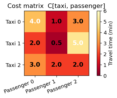
Three taxis wait at different spots in a city. Three passengers need rides. The cost matrix C[i, j] holds the travel time (in minutes) from taxi i to passenger j. We want to send each taxi to exactly one passenger and minimise total travel time.

This is the linear assignment problem (LAP): given a cost matrix, find the one-to-one assignment of rows to columns with minimum total cost.

# rows = taxis, columns = passengers
C = np.array(
    [
        [4.0, 1.0, 3.0],  # taxi 0: 4 min to p0, 1 min to p1, 3 min to p2
        [2.0, 0.5, 5.0],  # taxi 1: very close to p1
        [3.0, 2.0, 2.0],  # taxi 2: moderate distance to all
    ],
    dtype=np.float32,
)

labels_row = ["Taxi 0", "Taxi 1", "Taxi 2"]
labels_col = ["Passenger 0", "Passenger 1", "Passenger 2"]

fig, ax = plt.subplots(figsize=(5, 3))
im = ax.imshow(C, cmap="YlOrRd_r", vmin=0, vmax=6)
ax.set_xticks(range(3))
ax.set_yticks(range(3))
ax.set_xticklabels(labels_col, rotation=20, ha="right")
ax.set_yticklabels(labels_row)
plt.colorbar(im, ax=ax, label="Travel time (min)")
for i in range(3):
    for j in range(3):
        ax.text(
            j,
            i,
            f"{C[i, j]:.1f}",
            ha="center",
            va="center",
            fontsize=13,
            fontweight="bold",
            color="white" if C[i, j] > 3 else "black",
        )
ax.set_title("Cost matrix  C[taxi, passenger]")
plt.tight_layout()
plt.show()

Visualising the problem as a bipartite graph

An assignment problem always has this structure: two disjoint groups of items (taxis on the left, passengers on the right), with a potential connection — and a cost — between every item in the left group and every item in the right group. A valid assignment picks exactly one edge per left node and exactly one edge per right node (a perfect matching).

def draw_bipartite(ax, left_labels, right_labels, matching=None, costs=None, title=""):
    n = len(left_labels)
    left_x, right_x = 0.15, 0.85
    left_ys = np.linspace(0.85, 0.15, n)
    right_ys = np.linspace(0.85, 0.15, n)

    # all edges (grey, thin)
    for i, ly in enumerate(left_ys):
        for j, ry in enumerate(right_ys):
            ax.plot([left_x, right_x], [ly, ry], color="#cccccc", lw=0.8, zorder=1)
            if costs is not None:
                mx, my = (left_x + right_x) / 2, (ly + ry) / 2
                ax.text(
                    mx,
                    my,
                    f"{costs[i, j]:.1f}",
                    fontsize=7,
                    ha="center",
                    va="center",
                    color="#888888",
                )

    # matched edges (red, thick)
    if matching is not None:
        for i, j in enumerate(matching):
            ax.plot(
                [left_x, right_x],
                [left_ys[i], right_ys[j]],
                color="#E03520",
                lw=2.5,
                zorder=2,
            )

    # nodes
    for i, (y, lbl) in enumerate(zip(left_ys, left_labels)):
        ax.scatter(left_x, y, s=600, color="#1a6daf", zorder=3)
        ax.text(left_x - 0.04, y, lbl, ha="right", va="center", fontsize=10)
    for j, (y, lbl) in enumerate(zip(right_ys, right_labels)):
        ax.scatter(right_x, y, s=600, color="#d97706", zorder=3)
        ax.text(right_x + 0.04, y, lbl, ha="left", va="center", fontsize=10)

    ax.set_xlim(0, 1)
    ax.set_ylim(0, 1)
    ax.axis("off")
    ax.set_title(title)


fig, axes = plt.subplots(1, 2, figsize=(11, 4))
draw_bipartite(axes[0], labels_row, labels_col, costs=C, title="All possible edges")
# naive sequential assignment: taxi 0 → passenger 0, taxi 1 → passenger 1, etc.
naive = [0, 1, 2]
cost_naive = sum(C[i, j] for i, j in enumerate(naive))
draw_bipartite(
    axes[1],
    labels_row,
    labels_col,
    matching=naive,
    costs=C,
    title=f"Naïve assignment  (total = {cost_naive:.1f} min)",
)
plt.tight_layout()
plt.show()

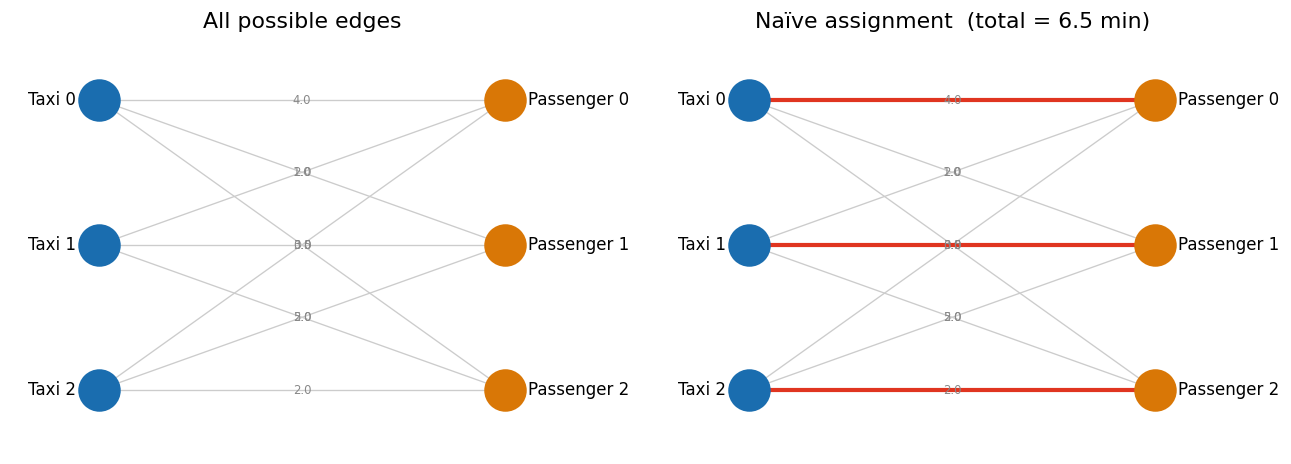
The naïve assignment (each taxi goes to the passenger with the same index) gives a higher total cost than necessary. Can we do better?

2 Why brute force does not scale

For n taxis and n passengers there are n! (n-factorial) possible assignments. For small problems we can check all of them; large problems defeat this approach.

def brute_force_lap(C):
    """Return the optimal assignment by checking every permutation."""
    n = C.shape[0]
    best_cost, best_perm = float("inf"), None
    for perm in permutations(range(n)):
        cost = sum(C[i, perm[i]] for i in range(n))
        if cost < best_cost:
            best_cost, best_perm = cost, list(perm)
    return best_perm, best_cost


opt_perm, opt_cost = brute_force_lap(C)
print(f"Optimal assignment : taxi {[i for i in range(3)]} → passenger {opt_perm}")
print(f"Optimal total cost : {opt_cost:.1f} min  (naïve was {cost_naive:.1f} min)")

Output

Optimal assignment : taxi [0, 1, 2] → passenger [1, 0, 2]
Optimal total cost : 5.0 min  (naïve was 6.5 min)

# Show how n! explodes
ns = list(range(1, 16))
factorials = [math.factorial(n) for n in ns]

fig, ax = plt.subplots(figsize=(7, 4))
ax.bar(ns, factorials, color="#4a90d9", edgecolor="white")
ax.set_yscale("log")
ax.set_xlabel("Problem size n  (number of items per side)")
ax.set_ylabel("Number of assignments to check  (log scale)")
ax.set_title("Brute-force search grows as n!")
ax.axhline(1e9, color="#E03520", ls="--", lw=1.5, label="10⁹  (≈ 1 second of CPU)")
ax.axhline(1e18, color="#b08800", ls="--", lw=1.5, label="10¹⁸  (≈ 30 years of CPU)")
ax.legend()
for i, (n, f) in enumerate(zip(ns, factorials)):
    if n in (5, 10, 13):
        ax.text(n, f * 2, f"n={n}\n{f:,}", ha="center", va="bottom", fontsize=8)
ax.set_xticks(ns)
plt.tight_layout()
plt.show()

print(f"n=10 → {math.factorial(10):,} permutations")
print(f"n=20 → {math.factorial(20):,} permutations  (infeasible)")

Output

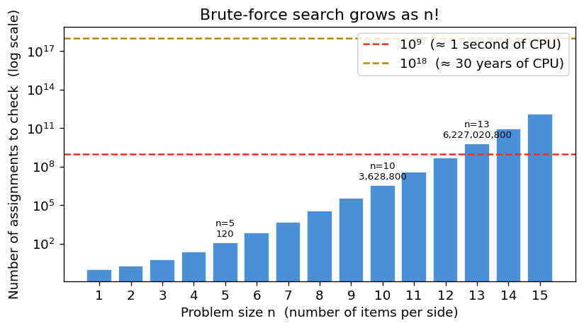
n=10 → 3,628,800 permutations
n=20 → 2,432,902,008,176,640,000 permutations  (infeasible)

Efficient algorithms (like the Hungarian method or Jonker-Volgenant) solve the LAP in O(n³) time — many orders of magnitude faster than brute force.

n	Brute force	O(n³)
10	3.6 million	1 000
100	~10¹⁵⁷	10⁶
1000	∞	10⁹

3 Solving with torchmatch

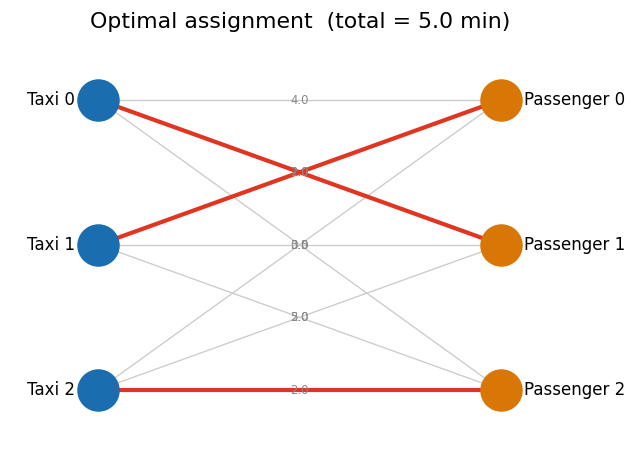
torchmatch.assignment.solve takes a 2-D (or 3-D batched) cost tensor and returns an integer tensor of length n_rows: element i is the column assigned to row i.

cost_t = torch.tensor(C)

row_to_col = torchmatch.assignment.solve(cost_t)
print("row_to_col :", row_to_col.tolist())
print("Optimal assignment:")
for taxi, passenger in enumerate(row_to_col.tolist()):
    print(f"  taxi {taxi}  →  passenger {passenger}  (cost {C[taxi, passenger]:.1f})")
total = cost_t[torch.arange(3), row_to_col].sum().item()
print(f"Total cost: {total:.1f}")

Output

row_to_col : [1, 0, 2]
Optimal assignment:
  taxi 0  →  passenger 1  (cost 1.0)
  taxi 1  →  passenger 0  (cost 2.0)
  taxi 2  →  passenger 2  (cost 2.0)
Total cost: 5.0

# Visualise the optimal matching
fig, ax = plt.subplots(figsize=(5.5, 4))
draw_bipartite(
    ax,
    labels_row,
    labels_col,
    matching=row_to_col.tolist(),
    costs=C,
    title=f"Optimal assignment  (total = {total:.1f} min)",
)
plt.tight_layout()
plt.show()

4 Rectangular problems and forbidden edges

Real problems are often rectangular (more items on one side than the other) or have forbidden pairs (some assignments are infeasible). torchmatch handles both.

# More taxis than passengers — some taxis stay idle (get assigned -1)
C_rect = torch.tensor(
    [
        [4.0, 1.0],
        [2.0, 0.5],
        [3.0, 2.0],
        [1.5, 3.5],  # extra taxi
    ],
    dtype=torch.float32,
)

result = torchmatch.assignment.solve(C_rect)
print("Rectangular (4 taxis, 2 passengers):", result.tolist())
print(" -1 means the taxi is unassigned")

# Forbidden edges: set to +inf
C_gated = torch.tensor(
    [
        [4.0, float("inf"), 3.0],  # taxi 0 cannot reach passenger 1
        [float("inf"), 0.5, 5.0],  # taxi 1 cannot reach passenger 0
        [3.0, 2.0, float("inf")],  # taxi 2 cannot reach passenger 2
    ],
    dtype=torch.float32,
)

result_gated = torchmatch.assignment.solve(C_gated)
print("\nWith forbidden edges (+inf):", result_gated.tolist())
total_gated = sum(
    C_gated[i, j].item()
    for i, j in enumerate(result_gated.tolist())
    if j >= 0 and C_gated[i, j] != float("inf")
)
print(f"Total feasible cost: {total_gated:.1f}")

Output

Rectangular (4 taxis, 2 passengers): [-1, 1, -1, 0]
 -1 means the taxi is unassigned

With forbidden edges (+inf): [2, 1, 0]
Total feasible cost: 6.5

5 Comparing to scipy

torchmatch produces the same optimal assignments as SciPy's reference solver, but stays inside the PyTorch ecosystem (no NumPy round-trip), supports batching, and runs on GPU.

# Verify correctness against scipy
scipy_rows, scipy_cols = linear_sum_assignment(C)
scipy_assignment = scipy_cols.tolist()
tm_assignment = torchmatch.assignment.solve(torch.tensor(C)).tolist()

print("scipy assignment :", scipy_assignment)
print("torchmatch       :", tm_assignment)
assert scipy_assignment == tm_assignment, "Mismatch!"
print("✓ Results match")

Output

scipy assignment : [1, 0, 2]
torchmatch       : [1, 0, 2]
✓ Results match

Summary

The linear assignment problem finds the minimum-cost one-to-one mapping between two sets of items.
Brute force is O(n!) and impractical for n > ~10.
torchmatch.assignment.solve(cost) solves in O(n³) using hardware-optimised kernels (AVX2 on CPU, CUDA on GPU).
Rectangular inputs and forbidden edges (+inf) are handled natively; unassigned rows return -1.

Next: Tutorial 2 — Backends and Batching explores the different solvers, when to choose each, and how to solve thousands of problems at once.

Tutorials

Interactive Jupyter notebooks covering both the assignment and transport families, from first principles through applied examples.

Tutorial 2 — Backends and Batching

What you will learn