

Tutorial 1 — What Is Optimal Transport?
What you will learn
Tutorial 1 — What Is Optimal Transport?
What you will learn
- The intuition behind optimal transport (OT) as "moving mass at minimum cost"
- How discrete OT relates to the assignment problem
- The Kantorovich formulation: a linear program over transport plans
- What a transport plan looks like and how to read it
- How to compute your first OT plan with
torchmatch.transport.matrix.solve
Prerequisites — Basic probability (distributions, histograms) and familiarity with NumPy arrays. No prior knowledge of OT is assumed.
%matplotlib inline
import matplotlib.pyplot as plt
import matplotlib.gridspec as gridspec
import numpy as np
import torch
import torchmatch

plt.rcParams.update({"figure.dpi": 120, "font.size": 11})
rng = np.random.default_rng(42)
print("torchmatch", torchmatch.__version__)
torchmatch 1.0.0
1 The earth-mover intuition
Imagine two piles of sand on a table. You want to rearrange the first pile so it looks like the second. Moving a grain of sand costs in proportion to the distance it travels. Optimal transport finds the cheapest way to move sand from the source pile to match the target pile.
In ML contexts:
- "Sand" is probability mass (or feature vectors, or pixels).
- The two piles are probability distributions
a(source) andb(target). - The cost of moving unit mass from point
x_ito pointy_jis given by a cost function (often squared Euclidean distance).
2 A 1-D example: two histograms
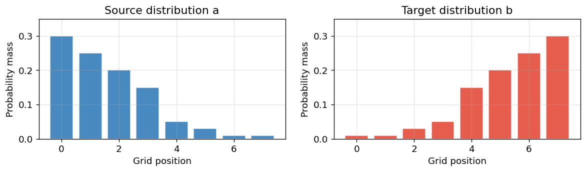
Start with the simplest possible case: two discrete distributions over a
1-D grid. The source a puts mass on the left; the target b puts mass
on the right. The optimal transport plan says exactly how to move mass.
N_BINS = 8  # grid points
grid = np.arange(N_BINS, dtype=np.float32)

# Source: mass concentrated on the left
a = np.array([0.30, 0.25, 0.20, 0.15, 0.05, 0.03, 0.01, 0.01], dtype=np.float32)
# Target: mass concentrated on the right
b = np.array([0.01, 0.01, 0.03, 0.05, 0.15, 0.20, 0.25, 0.30], dtype=np.float32)
assert np.isclose(a.sum(), 1.0) and np.isclose(b.sum(), 1.0)

# Cost matrix: squared Euclidean distance between grid points
C = (grid[:, None] - grid[None, :]) ** 2  # (8, 8)

fig, axes = plt.subplots(1, 2, figsize=(10, 3))
for ax, dist, title, color in zip(
    axes,
    [a, b],
    ["Source distribution a", "Target distribution b"],
    ["#1a6daf", "#E03520"],
):
    ax.bar(grid, dist, color=color, alpha=0.8, edgecolor="white")
    ax.set_xlabel("Grid position")
    ax.set_ylabel("Probability mass")
    ax.set_title(title)
    ax.set_ylim(0, 0.35)
    ax.grid(True, alpha=0.3)
plt.tight_layout()
plt.show()
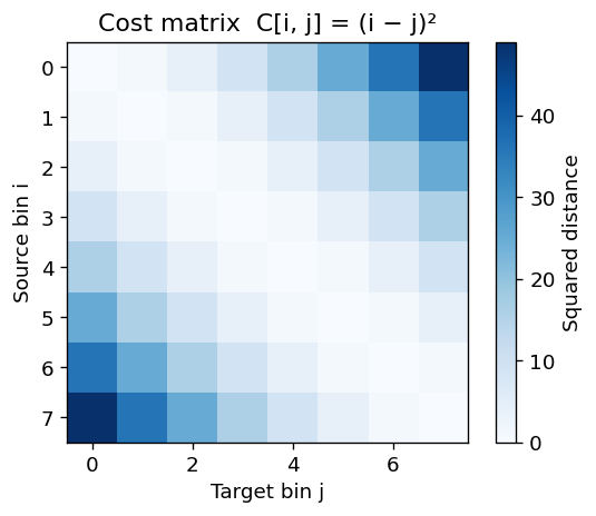
The cost matrix
C[i, j] = cost of moving one unit of mass from source bin i to target
bin j. Here cost = squared distance, so moving mass far costs more.
fig, ax = plt.subplots(figsize=(5, 4))
im = ax.imshow(C, cmap="Blues")
ax.set_xlabel("Target bin j")
ax.set_ylabel("Source bin i")
ax.set_title("Cost matrix  C[i, j] = (i − j)²")
plt.colorbar(im, ax=ax, label="Squared distance")
plt.tight_layout()
plt.show()
3 The transport plan
A transport plan P is an N × M matrix where P[i, j] is the
amount of mass moved from source bin i to target bin j. It must
satisfy two constraints:
- Source marginal: every row sums to
a[i](all source mass is shipped) - Target marginal: every column sums to
b[j](target receives the right mass)
The optimal plan minimises the total transport cost sum_{ij} P[i,j] * C[i,j].
OT is a generalisation of the assignment problem: when a and b are
both uniform (a[i] = b[j] = 1/N), the cheapest plan is always a
permutation matrix — exactly the assignment problem solution.
# Solve with torchmatch (default: entropic regularisation, reg=0.1)
cost_t = torch.tensor(C).unsqueeze(0)  # (1, 8, 8) — batch dimension required
a_t = torch.tensor(a).unsqueeze(0)  # (1, 8)
b_t = torch.tensor(b).unsqueeze(0)  # (1, 8)

log_plan = torchmatch.transport.matrix.solve(cost_t, a=a_t, b=b_t, reg=0.01, n_iter=500)
P = log_plan.exp().squeeze(0).numpy()  # (8, 8)

print(f"Plan shape: {P.shape}")
print(f"Row sums (should ≈ a): {P.sum(axis=1).round(3)}")
print(f"Col sums (should ≈ b): {P.sum(axis=0).round(3)}")
transport_cost = (P * C).sum()
print(f"Total transport cost: {transport_cost:.4f}")
Plan shape: (8, 8)
Row sums (should ≈ a): [0.05  0.111 0.089 0.338 0.112 0.18  0.06  0.06 ]
Col sums (should ≈ b): [0.01 0.01 0.03 0.05 0.15 0.2  0.25 0.3 ]
Total transport cost: 4.5030
fig, axes = plt.subplots(1, 2, figsize=(12, 4))

# Left: the plan as a heatmap
ax = axes[0]
im = ax.imshow(P, cmap="Reds", vmin=0)
ax.set_xlabel("Target bin j")
ax.set_ylabel("Source bin i")
ax.set_title("Transport plan  P[i, j]")
plt.colorbar(im, ax=ax, label="Mass transported")

# Right: the plan as flow arrows
ax = axes[1]
ax.bar(grid - 0.2, a, width=0.35, label="Source a", color="#1a6daf", alpha=0.7)
ax.bar(grid + 0.2, b, width=0.35, label="Target b", color="#E03520", alpha=0.7)

# Draw arrows proportional to mass moved
for i in range(N_BINS):
    for j in range(N_BINS):
        if P[i, j] > 0.005:
            ax.annotate(
                "",
                xy=(j + 0.2, 0),
                xytext=(i - 0.2, 0),
                arrowprops=dict(
                    arrowstyle="-|>",
                    color="#555555",
                    lw=P[i, j] * 8,
                    alpha=0.5,
                ),
            )

ax.set_xlabel("Grid position")
ax.set_ylabel("Probability mass")
ax.set_title("Mass flows  (arrow width ∝ amount moved)")
ax.legend()
ax.grid(True, alpha=0.3)
plt.tight_layout()
plt.show()
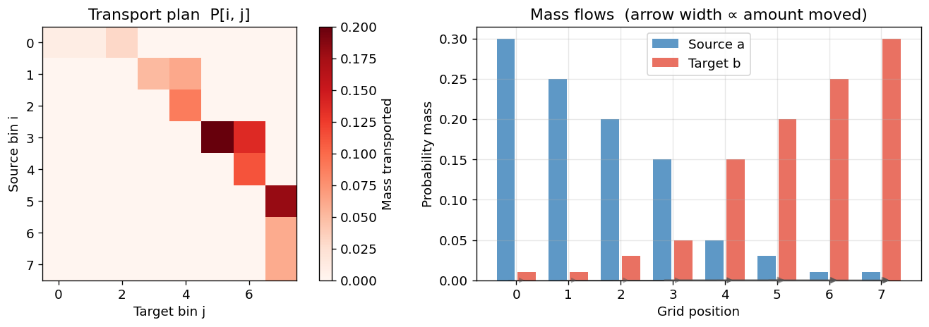
The plan moves mass from the left bins to the right bins in a "diagonal" pattern: nearby bins exchange more mass than distant ones, matching the squared-distance cost.
4 OT vs assignment: when they coincide
When both distributions are uniform (every bin has weight 1/N) and the
optimal plan turns out to be a permutation matrix, OT and LAP give the
same answer.
N = 5
a_unif = np.ones(N, dtype=np.float32) / N
b_unif = np.ones(N, dtype=np.float32) / N

# Cost: random non-symmetric
C_lap = rng.random((N, N)).astype(np.float32)
print("Cost matrix:")
print(C_lap.round(3))

# Solve as OT (should recover the same optimal permutation as LAP)
cost_lap = torch.tensor(C_lap).unsqueeze(0)
a_t_u = torch.tensor(a_unif).unsqueeze(0)
b_t_u = torch.tensor(b_unif).unsqueeze(0)

log_plan_unif = torchmatch.transport.matrix.solve(
    cost_lap, a=a_t_u, b=b_t_u, reg=0.001, n_iter=1000
)
P_unif = log_plan_unif.exp().squeeze(0).numpy()

# Also solve as LAP
assignment = torchmatch.assignment.solve(torch.tensor(C_lap))

print("\nOT plan (thresholded at 0.05):")
print((P_unif * N > 0.5).astype(int))  # permutation matrix

print("\nLAP assignment:", assignment.tolist())
print("LAP as permutation matrix:")
perm_matrix = np.zeros((N, N), dtype=int)
for i, j in enumerate(assignment.tolist()):
    perm_matrix[i, j] = 1
print(perm_matrix)
Cost matrix:
[[0.774 0.439 0.859 0.697 0.094]
 [0.976 0.761 0.786 0.128 0.45 ]
 [0.371 0.927 0.644 0.823 0.443]
 [0.227 0.555 0.064 0.828 0.632]
 [0.758 0.355 0.971 0.893 0.778]]

OT plan (thresholded at 0.05):
[[0 0 0 0 1]
 [0 0 0 1 0]
 [1 0 0 0 0]
 [0 0 1 0 0]
 [0 1 0 0 0]]

LAP assignment: [4, 3, 0, 2, 1]
LAP as permutation matrix:
[[0 0 0 0 1]
 [0 0 0 1 0]
 [1 0 0 0 0]
 [0 0 1 0 0]
 [0 1 0 0 0]]
With very small regularisation (reg=0.001), the OT plan approaches the
exact LAP solution. This is the key connection: assignment is OT between
uniform distributions with zero regularisation.
5 The Wasserstein distance
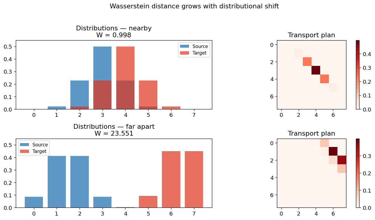
The Wasserstein distance (or earth mover's distance) is the minimum transport cost:
W(a, b) = min_P sum_{ij} P[i, j] * C[i, j]
Unlike the KL divergence or total variation, the Wasserstein distance respects the geometry of the underlying space: transporting mass farther costs more. This makes it a meaningful distance for comparing distributions over continuous spaces.
# Compare two pairs of distributions: one nearby, one far apart
def make_gaussian_hist(mean, std, n=8):
    grid = np.arange(n, dtype=np.float32)
    w = np.exp(-0.5 * ((grid - mean) / std) ** 2)
    return (w / w.sum()).astype(np.float32)


pairs = [
    (
        make_gaussian_hist(3.0, 0.8, N_BINS),
        make_gaussian_hist(4.0, 0.8, N_BINS),
        "nearby",
    ),
    (
        make_gaussian_hist(1.5, 0.8, N_BINS),
        make_gaussian_hist(6.5, 0.8, N_BINS),
        "far apart",
    ),
]

fig, axes = plt.subplots(2, 2, figsize=(11, 6))
for row, (ai, bi, label) in enumerate(pairs):
    cost_pair = torch.tensor(C).unsqueeze(0)
    log_p = torchmatch.transport.matrix.solve(
        cost_pair,
        a=torch.tensor(ai).unsqueeze(0),
        b=torch.tensor(bi).unsqueeze(0),
        reg=0.02,
        n_iter=300,
    )
    Pi = log_p.exp().squeeze(0).numpy()
    w_dist = (Pi * C).sum()

    axes[row, 0].bar(grid, ai, color="#1a6daf", alpha=0.7, label="Source")
    axes[row, 0].bar(grid, bi, color="#E03520", alpha=0.7, label="Target")
    axes[row, 0].set_title(f"Distributions — {label}\nW = {w_dist:.3f}")
    axes[row, 0].legend(fontsize=9)
    axes[row, 0].set_ylim(0, 0.55)

    im = axes[row, 1].imshow(Pi, cmap="Reds", vmin=0)
    axes[row, 1].set_title("Transport plan")
    plt.colorbar(im, ax=axes[row, 1])

plt.suptitle("Wasserstein distance grows with distributional shift", y=1.02)
plt.tight_layout()
plt.show()
Summary
- Optimal transport finds the minimum-cost way to "move" one probability distribution to match another.
- The solution is a transport plan
P[i, j]: the fraction of mass moved from sourceito targetj. - OT generalises the assignment problem: with uniform distributions and zero regularisation, the optimal plan is a permutation matrix.
- The Wasserstein distance measures how far apart two distributions are in a way that respects the geometry of the underlying space.
Next: Tutorial 2 — The Sinkhorn Algorithm explains why exact OT is expensive and how entropic regularisation makes large-scale OT practical.